


1. INTRODUCTION
Although advances in chemical characterization have reduced the reliance on bioassays for many products, bioassays are still essential for the determination of potency and the assurance of activity of many proteins, vaccines, complex mixtures, and products for cell and gene therapy, as well as for their role in monitoring the stability of biological products. The intended scope of general chapter Analysis of Biological Assays  1034
1034 includes guidance for the analysis of results both of bioassays described in the United States Pharmacopeia (USP), and of non-USP bioassays that seek to conform to the qualities of bioassay analysis recommended by USP. Note the emphasis on analysis—design and validation are addressed in complementary chapters (Development and Design of Bioassays 1032 and Biological Assay Validation 1033, respectively).
Topics addressed in 1034 include statistical concepts and methods of analysis for the calculation of potency and confidence intervals for a variety of relative potency bioassays, including those referenced in USP. Chapter 1034 is intended for use primarily by those who do not have extensive training or experience in statistics and by statisticians who are not experienced in the analysis of bioassays. Sections that are primarily conceptual require only minimal statistics background. Most of the chapter and all the methods sections require that the nonstatistician be comfortable with statistics at least at the level of USP general chapter Analytical Data—Interpretation and Treatment 1010 and with linear regression. Most of sections 3.4 Nonlinear Models for Quantitative Response and 3.6 Dichotomous (Quantal) Assays require more extensive statistics background and thus are intended primarily for statisticians. In addition, 1034 introduces selected complex methods, the implementation of which requires the guidance of an experienced statistician.
Approaches in 1034 are recommended, recognizing the possibility that alternative procedures may be employed. Additionally, the information in 1034 is presented assuming that computers and suitable software will be used for data analysis. This view does not relieve the analyst of responsibility for the consequences of choices pertaining to bioassay design and analysis.
2. OVERVIEW OF ANALYSIS OF BIOASSAY DATA
Following is a set of steps that will help guide the analysis of a bioassay. This section presumes that decisions were made following a similar set of steps during development, checked during validation, and then not required routinely. Those steps and decisions are covered in general information chapter Design and Development of Biological Assays 1032. Section 3 Analysis Models provides details for the various models considered.
- As a part of the chosen analysis, select the subset of data to be used in the determination of the relative potency using the prespecified scheme. Exclude only data known to result from technical problems such as contaminated wells, non-monotonic concentration–response curves, etc.
- Fit the statistical model for detection of potential outliers, as chosen during development, including any weighting and transformation. This is done first without assuming similarity of the Test and Standard curves but should include important elements of the design structure, ideally using a model that makes fewer assumptions about the functional form of the response than the model used to assess similarity.
- Determine which potential outliers are to be removed and fit the model to be used for suitability assessment. Usually, an investigation of outlier cause takes place before outlier removal. Some assay systems can make use of a statistical (noninvestigative) outlier removal rule, but removal on this basis should be rare. One approach to “rare” is to choose the outlier rule so that the expected number of false positive outlier identifications is no more than one; e.g., use a 1% test if the sample size is about 100. If a large number of outliers are found above that expected from the rule used, that calls into question the assay.
- Assess system suitability. System suitability assesses whether the assay Standard preparation and any controls behaved in a manner consistent with past performance of the assay. If an assay (or a run) fails system suitability, the entire assay (or run) is discarded and no results are reported other than that the assay (or run) failed. Assessment of system suitability usually includes adequacy of the fit of the model used to assess similarity. For linear models, adequacy of the model may include assessment of the linearity of the Standard curve. If the suitability criterion for linearity of the Standard is not met, the exclusion of one or more extreme concentrations may result in the criterion being met. Examples of other possible system suitability criteria include background, positive controls, max/min, max/background, slope, IC50 (or EC50), and variation around the fitted model.
- Assess sample suitability for each Test sample. This is done to confirm that the data for each Test sample satisfy necessary assumptions. If a Test sample fails sample suitability, results for that sample are reported as “Fails Sample Suitability.” Relative potencies for other Test samples in the assay may still be reported. Most prominent of sample suitability criteria is similarity, whether parallelism for parallel models or equivalence of intercepts for slope-ratio models. For nonlinear models, similarity assessment involves all curve parameters other than EC50 (or IC50).
- For those Test samples in the assay that meet the criterion for similarity to the Standard (i.e., sufficiently similar concentration–response curves or similar straight-line subsets of concentrations), calculate relative potency estimates assuming similarity between Test and Standard, i.e., by analyzing the Test and Standard data together using a model constrained to have exactly parallel lines or curves, or equal intercepts.
- A single assay is often not sufficient to achieve a reportable value, and potency results from multiple assays can be combined into a single potency estimate. Repeat steps 1–6 multiple times, as specified in the assay protocol or monograph, before determining a final estimate of potency and a confidence interval.
- Construct a variance estimate and a measure of uncertainty of the potency estimate (e.g., confidence interval). See section 4 Confidence Intervals.
A step not shown concerns replacement of missing data. Most modern statistical methodology and software do not require equal numbers at each combination of concentration and sample. Thus, unless otherwise directed by a specific monograph, analysts generally do not need to replace missing values.
3. ANALYSIS MODELS
A number of mathematical functions can be successfully used to describe a concentration–response relationship. The first consideration in choosing a model is the form of the assay response. Is it a number, a count, or a category such as Dead/Alive? The form will identify the possible models that can be considered.
Other considerations in choosing a model include the need to incorporate design elements in the model and the possible benefits of means models compared to regression models. For purposes of presenting the essentials of the model choices, section 3 Analysis Models assumes a completely randomized design so that there are no design elements to consider and presents the models in their regression form.
3.1 Quantitative and Qualitative Assay Responses
The terms quantitative and qualitative refer to the nature of the response of the assay used in constructing the concentration–response model. Assays with either quantitative or qualitative responses can be used to quantify product potency. Note that the responses of the assay at the concentrations measured are not the relative potency of the bioassay. Analysts should understand the differences among responses, concentration–response functions, and relative potency.
A quantitative response results in a number on a continuous scale. Common examples include spectrophotometric and luminescence responses, body weights and measurements, and data calculated relative to a standard curve (e.g., cytokine concentration). Models for quantitative responses can be linear or nonlinear (see sections 3.2–3.5).
A qualitative measurement results in a categorical response. For bioassay, qualitative responses are most often quantal, meaning they entail two possible categories such as Positive/Negative, 0/1, or Dead/Alive. Quantal responses may be reported as proportions (e.g., the proportion of animals in a group displaying a property). Quantal models are presented in section 3.6. Qualitative responses can have more than two possible categories, such as end-point titer assays. Models for more than two categories are not considered in this general chapter.
Assay responses can also be counts, such as number of plaques or colonies. Count responses are sometimes treated as quantitative, sometimes as qualitative, and sometimes models specific to integers are used. The choice is often based on the range of counts. If the count is mostly 0 and rarely greater than 1, the assay may be analyzed as quantal and the response is Any/None. If the counts are large and cover a wide range, such as 500 to 2500, then the assay may be analyzed as quantitative, possibly after transformation of the counts. A square root transformation of the count is often helpful in such analyses to better satisfy homogeneity of variances. If the range of counts includes or is near 0 but 0 is not the preponderant value, it may be preferable to use a model specific for integer responses. Poisson regression and negative binomial regression models are often good options. Models specific to integers will not be discussed further in this general chapter.
Assays with quantitative responses may be converted to quantal responses. For example, what may matter is whether some defined threshold is exceeded. The model could then be quantal—threshold exceeded or not. In general, assay systems have more precise estimates of potency if the model uses all the information in the response. Using above or below a threshold, rather than the measured quantitative responses, is likely to degrade the performance of an assay.
3.2 Overview of Models for Quantitative Responses
In quantitative assays, the measurement is a number on a continuous scale. Optical density values from plate-based assays are such measurements. Models for quantitative assays can be linear or nonlinear. Although the two display an apparent difference in levels of complexity, parallel-line (linear) and parallel-curve (nonlinear) models share many commonalities. Because of the different form of the equations, slope-ratio assays are considered separately (section 3.5 Slope-Ratio Concentration–Response Models).
Assumptions—
The basic parallel-line, parallel-curve, and slope-ratio models share some assumptions. All include a residual term, e, that represents error (variability) which is assumed to be independent from measurement to measurement and to have constant variance from concentration to concentration and sample to sample. Often the residual term is assumed to have a normal distribution as well. The assumptions of independence and equal variances are commonly violated, so the goal in analysis is to incorporate the lack of independence and the unequal variances into the statistical model or the method of estimation.
Lack of independence often arises because of the design or conduct of the assay. For example, if the assay consists of responses from multiple plates, observations from the same plate are likely to share some common influence that is not shared with observations from other plates. This is an example of intraplate correlation. A simple approach for dealing with this lack of independence is to include a block term in the statistical model for plate. With three or more plates this should be a random effects term so that we obtain an estimate of plate-to-plate variability.
In general, the model needs to closely reflect the design. The basic model equations given in sections 3.3–3.5 apply only to completely randomized designs. Any other design will mean additional terms in the statistical model. For example, if plates or portions of plates are used as blocks, one will need terms for blocks.
Calculation of Potency—
A primary assumption underlying methods used for the calculation of relative potency is that of similarity. Two preparations are similar if they contain the same effective constituent or same effective constituents in the same proportions. If this condition holds, the Test preparation behaves as a dilution (or concentration) of the Standard preparation. Similarity can be represented mathematically as follows. Let FT be the concentration–response function for the Test, and let FS be the concentration–response function for the Standard. The underlying mathematical model for similarity is:
 represents the relative potency of the Test sample relative to the Standard sample.
FT(z) = FS( z), [3.1]
[3.1]
where z represents the concentration and Methods for estimating in some common concentration–response models are discussed below. For linear models, the distinction between parallel-line models (section 3.3 Parallel-Line Models for Quantitative Response) and slope-ratio models (section 3.5 Slope-Ratio Concentration–Response Models) is based on whether a straight-line fit to log concentration or concentration yields better agreement between the model and the data over the range of concentrations of interest.
3.3 Parallel-Line Models for Quantitative Responses
In this section, a linear model refers to a concentration–response relationship, which is a straight-line (linear) function between the logarithm of concentration, x, and the response, y. y may be the response in the scale as measured or a transformation of the response. The functional form of this relationship is y = a + bx. Straight-line fits may be used for portions of nonlinear concentration–response curves, although doing so requires a method for selecting the concentrations to use for each of the Standard and Test samples (see 1032).
Means Model versus Regression—
A linear concentration–response model is most often analyzed with least squares regression. Such an analysis results in estimates of the unknown coefficients (intercepts and slope) and their standard errors, as well as measures of the goodness of fit [e.g., R2 and root-mean-square error (RMSE)].
Linear regression works best where all concentrations can be used and there is negligible curvature in the concentration–response data. Another statistical method for analyzing linear concentration–response curves is the means model. This is an analysis of variance (ANOVA) method that offers some advantages, particularly when one or more concentrations from one or more samples are not used to estimate potency. Because a means model includes a separate mean for each unique combination of sample and dose (as well as block or other effects associated with the design structure) it is equivalent to a saturated polynomial regression model. Hence, a means model provides an estimate of error that is independent of regression lack of fit. In contrast, a regression residual based estimate of error is a mixture of the assay error, as estimated by the means model, combined with lack of fit of the regression model. At least in this sense, the means model error is a better estimate of the residual error variation in an assay system.
Parallel-Line Concentration–Response Models—
If the general concentration–response model (3.1 Quantitative and Qualitative Assay Responses) can be made linear in x = log(z), the resulting equation is then:
 , and slope,
  , will differ between Test and Standard. With the parallelism (equal slopes) assumption, the model becomes
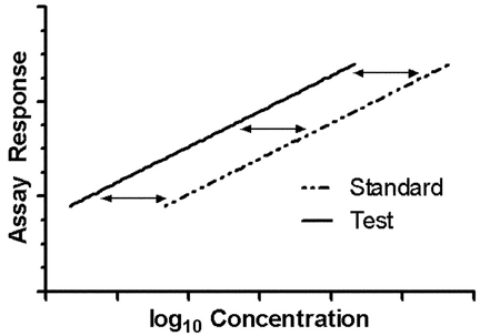
where S denotes Standard, T denotes Test, S = is the y-intercept for the Standard, and T = + log() is the y-intercept for the Test (see Figure 3.1).

y = + log(z) + e = + x + e,
where e is the residual or error term, and the intercept, | yS = |
[3.2] |
| yT = |
+'&img=../../images/v38332/c1034-f3-1.gif&casNumber=&usp=38&nf=33&chemicalStructureImage=false&ID='+parent.myID,600,500);)
Figure 3.1. Example of parallel-line model.
Where concentration–response lines are parallel, as shown in Figure 3.1, a separation or horizontal shift indicates a difference in the level of biological activity being assayed. This horizontal difference is numerically log(), the logarithm of the relative potency, and is found as the vertical distance between the lines T and S divided by the slope, . The relative potency is then
+'&img=../../images/v38332/c1034-eq1-ital-usp35.gif&casNumber=&usp=38&nf=33&chemicalStructureImage=false&ID='+parent.myID,600,500);)
Estimation of Parallel-line Models—
Parallel-line models are fit by the method of least squares. If the equal variance assumption holds, the parameters of equation [3.2] are chosen to minimize
 where the carets denote estimates. This is a linear regression with two independent variables, T and x, where T is a variable that equals 1 for observations from the Test and 0 for observations from the Standard. The summation in equation [3.3] is over all observations of the Test and Standard. If the equal variance assumption does not hold but the variance is known to be inversely proportional to a value, w, that does not depend on the current responses, the y's, and can be determined for each observation, then the method is weighted least squares


+'&img=../../images/v38332/c1034-eq3-3-ital-usp35.gif&casNumber=&usp=38&nf=33&chemicalStructureImage=false&ID='+parent.myID,600,500);)
+'&img=../../images/v38332/c1034-eq3-4italpf364.gif&casNumber=&usp=38&nf=33&chemicalStructureImage=false&ID='+parent.myID,600,500);)
Equation 3.4 is appropriate only if the weights are determined without using the response, the y's, from the current data (see 1032 for guidance in determining weights). In equations [3.3] and [3.4] is the same as the in equation [3.2] and  = T
= T  S = log . So, the estimate of the relative potency, , is
+'&img=../../images/v38332/c1034-eq2-ital-usp35.gif&casNumber=&usp=38&nf=33&chemicalStructureImage=false&ID='+parent.myID,600,500);)
Commonly available statistical software and spreadsheets provide routines for least squares. Not all software can provide weighted analyses.
See section 4 for methods to obtain a confidence interval for the estimated relative potency. For a confidence interval based on combining relative potency estimates from multiple assays, use the methods of section 4.2. For a confidence interval from a single assay, use Fieller’s Theorem (section 4.3) applied to  .
.
;) .
.
Measurement of Nonparallelism—
Parallelism for linear models is assessed by considering the difference or ratio of the two slopes. For the difference, this can be done by fitting the regression model,
= T S,  = T S, and T = 1 for Test data and T = 0 for Standard data. Then use the standard t-distribution confidence interval for . For the ratio of slopes, fit
T/S.
= T S, and T = 1 for Test data and T = 0 for Standard data. Then use the standard t-distribution confidence interval for . For the ratio of slopes, fit
T/S.
y = S + T + Sx + xT + e
where y = S + T + Sx(1 T) + TxT + e
and use Fieller’s Theorem, equation [4.3], to obtain a confidence interval for
3.4 Nonlinear Models for Quantitative Responses
Nonlinear concentration–response models are typically S-shaped functions. They occur when the range of concentrations is wide enough so that responses are constrained by upper and lower asymptotes. The most common of these models is the four-parameter logistic function as given below.
Let y denote the observed response and z the concentration. One form of the four-parameter logistic model is
+'&img=../../images/v38332/c1034-eq3-5.gif&casNumber=&usp=38&nf=33&chemicalStructureImage=false&ID='+parent.myID,600,500);)
+'&img=../../images/v38332/c1034-eq3-6pf364.gif&casNumber=&usp=38&nf=33&chemicalStructureImage=false&ID='+parent.myID,600,500);)
The two forms correspond as follows:
Lower asymptote: D = a0
Upper asymptote: A = a0 + d
Steepness: B = M (related to the slope of the curve at the EC50)
Effective concentration 50% (EC50): C = antilog(b) (may also be termed ED50).
Any convenient base for logarithms is suitable; it is often convenient to work in log base 2, particularly when concentrations are twofold apart.
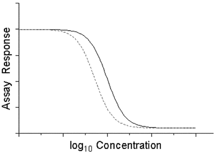
The four-parameter logistic curve is symmetric around the EC50 when plotted against log concentration because the rates of approach to the upper and lower asymptotes are the same (see Figure 3.2). For assays where this symmetry does not hold, asymmetrical model functions may be applied. These models are not considered further in this general chapter.
+'&img=../../images/v38332/c1034-f3-2.gif&casNumber=&usp=38&nf=33&chemicalStructureImage=false&ID='+parent.myID,600,500);)
Figure 3.2. Examples of symmetric (four-parameter logistic) and asymmetric sigmoids.
In many assays the analyst has a number of strategic choices to make during assay development (see Development and Design of Biological Assays 1032). For example, the responses could be modeled using a transformed response to a four-parameter logistic curve, or the responses could be weighted and fit to an asymmetric sigmoid curve. Also, it is often important to include terms in the model (often random effects) to address variation in the responses (or parameters of the response) associated with blocks or experimental units in the design of the assay. For simple assays where observations are independent, these strategic choices are fairly straightforward. For assays performed with grouped dilutions (as with multichannel pipets), assays with serial dilutions, or assay designs that include blocks (as with multiple plates per assay), it is usually a serious violation of the statistical assumptions to ignore the design structure. For such assays, a good approach involves a transformation that approximates a solution to non-constant variance, non-normality, and asymmetry combined with a model that captures the important parts of the design structure.
Parallel-Curve Concentration–Response Models—
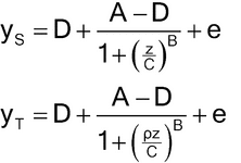
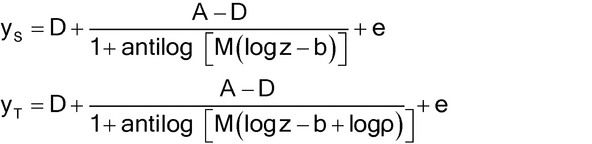
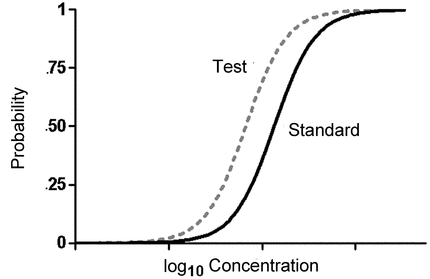
The concept of parallelism is not restricted to linear models. For nonlinear curves, parallel or similar means the concentration–response curves can be superimposed following a horizontal displacement of one of the curves, as shown in Figure 3.3 for four-parameter logistic curves. In terms of the parameters of equation [3.5], this means the values of A, D, and B for the Test are the same as for the Standard.
+'&img=../../images/v38332/c1034-f3-3.gif&casNumber=&usp=38&nf=33&chemicalStructureImage=false&ID='+parent.myID,600,500);)
Figure 3.3. Example of parallel curves from a nonlinear model.
The equations corresponding to the figure (with error term, e, added) are
+'&img=../../images/v38332/c1034-eq3-8.gif&casNumber=&usp=38&nf=33&chemicalStructureImage=false&ID='+parent.myID,600,500);)
or
+'&img=../../images/v38332/c1034-eq3-9-usp35.gif&casNumber=&usp=38&nf=33&chemicalStructureImage=false&ID='+parent.myID,600,500);)
Log is the log of the relative potency and the horizontal distance between the two curves, just as for the parallel-line model. Because the EC50 of the standard is antilog(b) and that of the Test is antilog(b log ) = antilog(b)/, the relative potency is the ratio of EC50’s (standard over Test) when the parallel-curve model holds.
Estimation of Parallel-Curve Models—
Estimation of nonlinear, parallel-curve models is similar to that for parallel-line models, possibly after transformation of the response and possibly with weighting. For the four-parameter logistic model, the parameter estimates are found by minimizing:
 without weighting, or
 with weighting. (As for equation [3.4], equation [3.6] is appropriate only if the weights are determined without using the responses, y's, from the current data.) In either case, the estimate of r is the estimate of the log of the relative potency. For some software, it may be easier to work with d = A D.
+'&img=../../images/v38332/c1034-eq3-10pf364.gif&casNumber=&usp=38&nf=33&chemicalStructureImage=false&ID='+parent.myID,600,500);)
+'&img=../../images/v38332/c1034-eq3-11pf364.gif&casNumber=&usp=38&nf=33&chemicalStructureImage=false&ID='+parent.myID,600,500);)
The parameters of the four-parameter logistic function and those of the asymmetric sigmoid models cannot be found with ordinary (linear) least squares regression routines. Computer programs with nonlinear estimation techniques must be used.
Analysts should not use the nonlinear regression fit to assess parallelism or estimate potency if any of the following are present: a) inadequate asymptote information is available; or b) a comparison of pooled error(s) from nonlinear regression to pooled error(s) from a means model shows that the nonlinear model does not fit well; or c) other appropriate measures of goodness of fit show that the nonlinear model is not appropriate (e.g., residual plots show evidence of a “hook”).
See section 4 for methods to obtain a confidence interval for the estimated relative potency. For a confidence interval based on combining relative potency estimates from multiple assays, use the methods of section 4.2. For a confidence interval from a single assay, advanced techniques, such as likelihood profiles or bootstrapping are needed to obtain a confidence interval for the log relative potency, r.
Measurement of Nonparallelism—
Assessment of parallelism for a four-parameter logistic model means assessing the slope parameter and the two asymptotes. During development (see 1032), a decision should be made regarding which parameters are important and how to measure nonparallelism. As discussed in 1032, the measure of nonsimilarity may be a composite measure that considers all parameters together in a single measure, such as the parallelism sum of squares (see 1032), or may consider each parameter separately. In the latter case, the measure may be functions of the parameters, such as an asymptote divided by the difference of asymptotes or the ratio of the asymptotes. For each parameter (or function of parameters), confidence intervals can be computed by bootstrap or likelihood profile methods. These methods are not presented in this general chapter.
3.5 Slope-Ratio Concentration–Response Models
If a straight-line regression fits the nontransformed concentration–response data well, a slope-ratio model may be used. The equations for the slope-ratio model assuming similarity are then:
| yS = |
[3.7] |
| yT = |
An identifying characteristic of a slope-ratio concentration–response model that can be seen in the results of a ranging study is that the lines for different potencies from a ranging study have the same intercept and different slopes. Thus, a graph of the ranging study resembles a fan. Figure 3.4 shows an example of a slope-ratio concentration–response model. Note that the common intercept need not be at the origin.
+'&img=../../images/v38332/c1034-f3-4.gif&casNumber=&usp=38&nf=33&chemicalStructureImage=false&ID='+parent.myID,600,500);)
Figure 3.4. Example of slope-ratio model.
An assay with a slope-ratio concentration–response model for measuring relative potency consists, at a minimum, of one Standard sample and one Test sample, each measured at one or more concentrations and, usually, a measured response with no sample (zero concentration). Because the concentrations are not log transformed, they are typically equally spaced on the original, rather than log, scale. The model consists of one common intercept, a slope for the Test sample results, and a slope for the Standard sample results as in equation [3.7]. The relative potency is then found from the ratio of the slopes:
Relative Potency = Test sample slope/Standard sample slope = / =
Assumptions for and Estimation of Slope-Ratio Models—
The assumptions for the slope-ratio model are the same as for parallel-line models: The residual terms are independent, have constant variance, and may need to have a normal distribution. The method of estimation is also least squares. This may be implemented either with or without weighting, as demonstrated in equations [3.8] and [3.9], respectively.


+'&img=../../images/v38332/c1034-eq3-14-usp35.gif&casNumber=&usp=38&nf=33&chemicalStructureImage=false&ID='+parent.myID,600,500);)
+'&img=../../images/v38332/c1034-eq3-15-usp35.gif&casNumber=&usp=38&nf=33&chemicalStructureImage=false&ID='+parent.myID,600,500);)
Equation [3.9] is appropriate only if the weights are determined without using the response, the y's, from the current data. This is a linear regression with two independent variables, z(1 T) and zT, where T = 1 for Test data and T = 0 for Standard data.  is the estimated slope for the Test,
  the estimated slope for the Standard, and then the estimate of relative potency is
+'&img=../../images/v38332/c1034-betarpf364.gif&casNumber=&usp=38&nf=33&chemicalStructureImage=false&ID='+parent.myID,600,500);)
Because the slope-ratio model is a linear regression model, most statistical packages and spreadsheets can be used to obtain the relative potency estimate. In some assay systems, it is sometimes appropriate to omit the zero concentration (e.g., if the no-dose controls are handled differently in the assay) and at times one or more of the high concentrations (e.g., if there is a hook effect where the highest concentrations do not have the highest responses). The discussion about using a means model and selecting subsets of concentrations for straight parallel-line bioassays applies to slope-ratio assays as well.
See section 4 for methods to obtain a confidence interval for the estimated relative potency. For a confidence interval based on combining relative potency estimates from multiple assays, use the methods of section 4.2. For a confidence interval from a single assay, use Fieller’s Theorem (section 4.3) applied to
+'&img=../../images/v38332/c1034-eqb-usp35.gif&casNumber=&usp=38&nf=33&chemicalStructureImage=false&ID='+parent.myID,600,500);)
Measurement of Nonsimilarity—
For slope-ratio models, statistical similarity corresponds to equal intercepts for the Standard and Test. To assess the similarity assumption it is necessary to have at least two nonzero concentrations for each sample. If the intercepts are not equal, equation [3.7] becomes
Departure from similarity is typically measured by the difference of intercepts, T S. An easy way to obtain a confidence interval is to fit the model,
= T S and use the standard t-distribution-based confidence interval for .
| yS = |
| yT = |
y = S + T + Sz(1 T) + TzT + e,
where
3.6 Dichotomous (Quantal) Assays
For quantal assays the assay measurement has a dichotomous or binary outcome, e.g., in animal assays the animal is dead or alive or a certain physiologic response is or is not observed. For cellular assays, the quantal response may be whether there is or is not a response beyond some threshold in the cell. In cell-based viral titer or colony-forming assays, the quantal response may be a limit of integer response such as an integer number of particles or colonies. When one can readily determine if any particles are present—but not their actual number—then the assay can be analyzed as quantal. Note that if the reaction can be quantitated on a continuous scale, as with an optical density, then the assay is not quantal.
Models for Quantal Analyses—
The key to models for quantal responses is to work with the probability of a response (e.g., probability of death), in contrast to quantitative responses for which the model is for the response itself. For each concentration, z, a treated animal, as an example, has a probability of responding to that concentration, P(z). Often the curve P(z) can be approximated by a sigmoid when plotted against the logarithm of concentration, as shown in Figure 3.5. This curve shows that the probability of responding increases with concentration. The concentration that corresponds to a probability of 0.5 is the EC50.
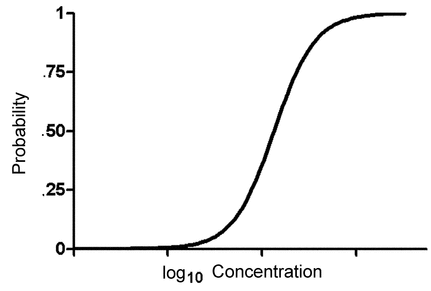
+'&img=../../images/v38332/c1034-f3-5.gif&casNumber=&usp=38&nf=33&chemicalStructureImage=false&ID='+parent.myID,600,500);)
Figure 3.5. Example of sigmoid for P(z).
The sigmoid curve is usually modeled based on the normal or logistic distribution. If the normal distribution is used, the resulting analysis is termed probit analysis, and if the logistic is used the analysis is termed logit or logistic analysis. The probit and logit models are practically indistinguishable, and either is an acceptable choice. The choice may be based on the availability of software that meets the laboratory’s analysis and reporting needs. Because software is more commonly available for logistic models (often under the term logistic regression) this discussion will focus on the use and interpretation of logit analysis. The considerations discussed in this section for logit analysis (using a logit transformation) apply as well to probit analysis (using a probit transformation).
Logit Model—
The logit model for the probability of response, P(z), can be expressed in two equivalent forms. For the sigmoid,
 where log(ED50) = 0/1. An alternative form shows the relationship to linear models:


+'&img=../../images/v38332/c1034-eq3-16-usp35.gif&casNumber=&usp=38&nf=33&chemicalStructureImage=false&ID='+parent.myID,600,500);)
+'&img=../../images/v38332/c1034-eq3-17-usp35.gif&casNumber=&usp=38&nf=33&chemicalStructureImage=false&ID='+parent.myID,600,500);)
The linear form is usually shown using natural logs and is a useful reminder that many of the considerations, in particular linearity and parallelism, discussed for parallel-line models in section 3.3 Parallel-Line Models for Quantitative Responses apply to quantal models as well.
For a logit analysis with Standard and Test preparations, let T be a variable that takes the value 1 for animals receiving the Test preparation and 0 for animals receiving the Standard. Assuming parallelism of the Test and Standard curves, the logit model for estimating relative potency is then:
+'&img=../../images/v38332/c1034-eq3-18-usp35.gif&casNumber=&usp=38&nf=33&chemicalStructureImage=false&ID='+parent.myID,600,500);)
The log of the relative potency of the Test compared to the Standard preparation is then 2/1. The two curves in Figure 3.6 show parallel Standard and Test sigmoids. (If the corresponding linear forms equation [3.10] were shown, they would be two parallel straight lines.) The log of the relative potency is the horizontal distance between the two curves, in the same way as for the linear and four-parameter logistic models given for quantitative responses (sections 3.3 Parallel-Line Models for Quantitative Responses and 3.4 Nonlinear Models for Quantitative Responses).
+'&img=../../images/v38332/c1034-f3-6.gif&casNumber=&usp=38&nf=33&chemicalStructureImage=false&ID='+parent.myID,600,500);)
Figure 3.6. Example of Parallel Sigmoid Curves.
Estimating the Model Parameters and Relative Potency—
Two methods are available for estimating the parameters of logit and probit models: maximum likelihood and weighted least squares. The difference is not practically important, and the laboratory can accept the choice made by its software. The following assumes a general logistic regression software program. Specialized software should be similar.

Considering the form of equation [3.10], one observes a resemblance to linear regression. There are two independent variables, x = log(z) and T. For each animal, there is a yes/no dependent variable, often coded as 1 for yes or response and 0 for no or no response. Although bioassays are often designed with equal numbers of animals per concentration, that is not a requirement of analysis. Utilizing the parameters estimated by software, which include 0, 1, and 2 and their standard errors, one obtains the estimate of the natural log of the relative potency:
+'&img=../../images/v38332/c1034-eq3-19italpf364.gif&casNumber=&usp=38&nf=33&chemicalStructureImage=false&ID='+parent.myID,600,500);)
See section 4 for methods to obtain a confidence interval for the estimated relative potency. For a confidence interval based on combining relative potency estimates from multiple assays, use the methods of section 4.2. For a confidence interval from a single assay, use Fieller’s Theorem (section 4.3) applied to  . The confidence interval for the relative potency is then [antilog(L), antilog(U)], where [L, U] is the confidence interval for the log relative potency.
;) . The confidence interval for the relative potency is then [antilog(L), antilog(U)], where [L, U] is the confidence interval for the log relative potency.
. The confidence interval for the relative potency is then [antilog(L), antilog(U)], where [L, U] is the confidence interval for the log relative potency.
Assumptions—
Assumptions for quantal models have two parts. The first concerns underlying assumptions related to the probability of response of each animal or unit in the bioassay. These are difficult to verify assumptions that depend on the design of the assay. The second part concerns assumptions for the statistical model for P(z). Most important of these are parallelism and linearity. These assumptions can be checked much as for parallel-line analyses for quantitative responses.
In most cases, quantal analyses assume a standard binomial probability model, a common choice of distribution for dichotomous data. The key assumptions of the binomial are that at a given concentration each animal treated at that concentration has the same probability of responding and the results for any animal are independent from those of all other animals. This basic set of assumptions can be violated in many ways. Foremost among them is the presence of litter effects, where animals from the same litter tend to respond more alike than do animals from different litters. Cage effects, in which the environmental conditions or care rendered to any specific cage makes the animals from that cage more or less likely to respond to experimental treatment, violates the equal-probability and independence assumptions. These assumption violations and others like them (that could be a deliberate design choice) do not preclude the use of logit or probit models. Still, they are indications that a more complex approach to analysis than that presented here may be required (see 1032).
Checking Assumptions—
The statistical model for P(z) assumes linearity and parallelism. To assess parallelism, equation [3.10] may be modified as follows:
 Here, 3 is the difference of slopes between Test and Standard and should be sufficiently small. [The T*log(z) term is known as an interaction term in statistical terminology.] The measure of nonparallelism may also be expressed in terms of the ratio of slopes, (1 + 3)/1. For model-based confidence intervals for these measures of nonparallelism, bootstrap or profile likelihood methods are recommended. These methods are not covered in this general chapter.
+'&img=../../images/v38332/c1034-eq3-20-usp35.gif&casNumber=&usp=38&nf=33&chemicalStructureImage=false&ID='+parent.myID,600,500);)
To assess linearity, it is good practice to start with a graphical examination. In accordance with equation [3.10], this would be a plot of log[(y + 0.5)/(n y + 0.5)] against log(concentration), where y is the total number of responses at the concentration and n is the number of animals at that concentration. (The 0.5 corrections improve the properties of this calculation as an estimate of log[P/(1 P)].) The lines for Test and Standard should be parallel straight lines as for the linear model in quantitative assays. If the relationship is monotonic but does not appear to be linear, then the model in [3.10] can be extended with other terms. For example, a quadratic term in log(concentration) could be added: [log(concentration)]2. If concentration needs to be transformed to something other than log concentration, then the quantal model analogue of slope-ratio assays is an option. The latter is possible but sufficiently unusual that it will not be discussed further in this general chapter.
Outliers—
Assessment of outliers is more difficult for quantal assays than for quantitative assays. Because the assay response can be only yes or no, no individual response can be unusual. What may appear to fall into the outlier category is a single response at a low concentration or a single no-response at a high concentration. Assuming that there has been no cause found (e.g., failure to properly administer the drug to the animal), there is no statistical basis for distinguishing an outlier from a rare event.
Alternative Methods—
Alternatives to the simple quantal analyses outlined here may be acceptable, depending on the nature of the analytical challenge. One such challenge is a lack of independence among experimental units, as may be seen in litter effects in animal assays. Some of the possible approaches that may be employed are Generalized Estimating Equations (GEE), generalized linear models, and generalized linear mixed-effects models. A GEE analysis will yield standard errors and confidence intervals whose validity does not depend on the satisfaction of the independence assumption.
There are also methods that make no particular choice of the model equation for the sigmoid. A commonly seen example is the Spearman–Kärber method.
4. CONFIDENCE INTERVALS
A report of an assay result should include a measure of the uncertainty of that result. This is often a standard error or a confidence interval. An interval (c, d), where c is the lower confidence limit and d is the upper confidence limit, is a 95% confidence interval for a parameter (e.g., relative potency) if 95% of such intervals upon repetition of the experiment would include the actual value of the parameter. A confidence interval may be interpreted as indicating values of the parameter that are consistent with the data. This interpretation of a confidence interval requires that various assumptions be satisfied. Assumptions also need to be satisfied when the width or half width [(d-c)/2] is used in a monograph as a measure of whether there is adequate precision to report a potency. The interval width is sometimes used as a suitability criterion without the confidence interpretation. In such cases the assumptions need not be satisfied.
Confidence intervals can either be model-based or sample-based. A model-based interval is based on the standard errors for each of the one or more estimates of log relative potency that come from the analysis of a particular statistical model. Model-based intervals should be avoided if sample-based intervals are possible. Model-based intervals require that the statistical model correctly incorporate all the effects and correlations that influence the model’s estimate of precision. These include but are not be limited to serial dilution and plate effects. Section 4.3 Model-Based Methods describes Fieller’s Theorem, a commonly used model-based interval.
Sample-based methods combine independent estimates of log relative potency. Multiple assays may arise because this was determined to be required during development and validation or because the assay procedure fixes a maximum acceptable width of the confidence interval and two or more independent assays may be needed to meet the specified width requirement. Some sample-based methods do not require that the statistical model correctly incorporate all effects and correlations. However, this should not be interpreted as dismissing the value of addressing correlations and other factors that influence within-assay precision. The within-assay precision is used in similarity assessment and is a portion of the variability that is the basis for the sample-based intervals. Thus minimizing within-assay variability to the extent practical is important. Sample-based intervals are covered in section 4.2 Combining Independent Assays (Sample-Based Confidence Interval Methods).
4.1 Combining Results from Multiple Assays
In order to mitigate the effects of variability, it is appropriate to replicate independent bioassays and combine their results to obtain a single reportable value. That single reportable value (and not the individual assay results) is then compared to any applicable acceptance criteria. During assay development and validation, analysts should evaluate whether it is useful to combine the results of such assays and, if so, in what way to proceed.
There are two primary questions to address when considering how to combine results from multiple assays:
Are the assays mutually independent?
A set of assays may be regarded as mutually independent when the responses of one do not in any way depend on the distribution of responses of any of the others. This implies that the random errors in all essential factors influencing the result (for example, dilutions of the standard and of the preparation to be examined or the sensitivity of the biological indicator) in one assay must be independent of the corresponding random errors in the other assays. Assays on successive days using the original and retained dilutions of the Standard, therefore, are not independent assays. Similarly, if the responses, particularly the potency, depend on other reagents that are shared by assays (e.g., cell preparations), the assays may not be independent.
Assays need not be independent in order for analysts to combine results. However, methods for independent assays are much simpler. Also, combining dependent assay results may require assumptions about the form of the correlation between assay results that may be, at best, difficult to verify. Statistical methods are available for dependent assays, but they are not presented in this general chapter.
Are the results of the assays homogeneous?
Homogeneous results differ only because of random within-assay errors. Any contribution from factors associated with intermediate precision precludes homogeneity of results. Intermediate precision factors are those that vary between assays within a laboratory and can include analyst, equipment, and environmental conditions. There are statistical tests for heterogeneity, but lack of statistically significant heterogeneity is not properly taken as assurance of homogeneity and so no test is recommended. If analysts use a method that assumes homogeneity, homogeneity should be assessed during development, documented during validation, and monitored during ongoing use of the assay.
Additionally, before results from assays can be combined, analysts should consider the scale on which that combination is to be made. In general, the combination should be done on the scale for which the parameter estimates are approximately normally distributed. Thus, for relative potencies based on a parallel-line, parallel-curve, or quantal method, the relative potencies are combined in the logarithm scale.
4.2 Combining Independent Assays (Sample-Based Confidence Interval Methods)
Analysts can use several methods for combining the results of independent assays. A simple method described below (Method 1) assumes a common distribution of relative potencies across the assays and is recommended. A second procedure is provided and may be useful if homogeneity of relative potency across assays can be documented. A third alternative is useful if the assumptions for Methods 1 and 2 are not satisfied. Another alternative, analyzing all assays together using a linear or nonlinear mixed-effects model, is not discussed in this general chapter.
Method 1—Independent Assay Results from a Common Assay Distribution—
The following is a simple method that assumes independence of assays. It is assumed that the individual assay results (logarithms of relative potencies) are from a common normal distribution with some nonzero variance. This common distribution assumption requires that all assays to be combined used the same design and laboratory procedures. Implicit is that the relative potencies may differ between the assays. This method thus captures interassay variability in relative potency. Note that the individual relative potencies should not be rounded before combining results.
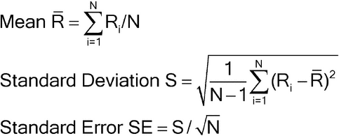

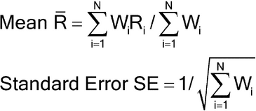
Let Ri denote the logarithm of the relative potency of the ith assay of N assay results to be combined. To combine the N results, the mean, standard deviation, and standard error of the Ri are calculated in the usual way:
+'&img=../../images/v38332/c1034-eq5-usp35.gif&casNumber=&usp=38&nf=33&chemicalStructureImage=false&ID='+parent.myID,600,500);)
A 100(1 )% confidence interval is then found as
R ± tN 1,/2SE,
where tN 1,/2 is the upper /2 percentage point of a t-distribution with N 1 degrees of freedom. The quantity tN 1,/2SE is the expanded uncertainty of R. The number, N, of assays to be combined is usually small, and hence the value of t is usually large.
Because the results are combined in the logarithm scale, the combined result can be reported in the untransformed scale as a confidence interval for the geometric mean potency, estimated by antilog(R),
+'&img=../../images/v38332/c1034eqanti-usp35.gif&casNumber=&usp=38&nf=33&chemicalStructureImage=false&ID='+parent.myID,600,500);)
Method 2—Independent Assay Results, Homogeneity Assumed—
This method can be used provided the following conditions are fulfilled:
- The individual potency estimates form a homogeneous set with regard to the potency being estimated. Note that this means documenting (usually during development and validation) that there are no contributions to between-assay variability from intermediate precision factors. The individual results should appear to be consistent with homogeneity. In particular, differences between them should be consistent with their standard errors.
- The potency estimates are derived from independent assays.
- The number of degrees of freedom of the individual residual errors is not small. This is required so that the weights are well determined.
When these conditions are not fulfilled, this method cannot be applied and Method 1, Method 3, or some other method should be used. Further note that Method 2 (because it assumes no inter-assay variability) often results in narrower confidence intervals than Method 1, but this is not sufficient justification for using Method 2 absent satisfaction of the conditions listed above.
Calculation of Weighting Coefficients—
It is assumed that the results of each of the N assays have been analyzed to give N estimates of log potency with associated confidence limits. For each assay, i, the logarithmic confidence interval for the log potency or log relative potency and a value Li are obtained by subtracting the lower confidence limit from the upper. (This formula, using the Li, accommodates asymmetric confidence intervals such as from Fieller’s Theorem, section 4.3 Model-Based Methods). A weight Wi for each value of the log relative potency, Ri, is calculated as follows, where ti has the same value as that used in the calculation of confidence limits in the ith assay:

+'&img=../../images/v38332/c1034-eq4-1.gif&casNumber=&usp=38&nf=33&chemicalStructureImage=false&ID='+parent.myID,600,500);)
Calculation of the Weighted Mean and Confidence Limits—
The products WiRi are formed for each assay, and their sum is divided by the total weight for all assays to give the weighted mean log relative potency and its standard error as follows:

+'&img=../../images/v38332/c1034-eq6.gif&casNumber=&usp=38&nf=33&chemicalStructureImage=false&ID='+parent.myID,600,500);)
A 100(1 )% confidence interval in the log scale is then found as
+'&img=../../images/v38332/c1034-fig4_2-2susp36.gif&casNumber=&usp=38&nf=33&chemicalStructureImage=false&ID='+parent.myID,600,500);)
where tk,/2 is the upper /2 percentage point of a t-distribution with degrees of freedom, k, equal to the sum of the number of degrees of freedom for the error mean squares in the individual assays. This confidence interval can then be transformed back to the original scale as for Method 1.
Method 3—Independent Assay Results, Common Assay Distribution Not Assumed—
Method 3 is an approximate method that may be considered if the conditions for Method 1 (common assay distribution) or Method 2 (homogeneity) are not met.

The observed variation then has two components:
-
the intra-assay variation for assay i:

-
the inter-assay variation:

+'&img=../../images/v38332/c1034-eq20pf364.gif&casNumber=&usp=38&nf=33&chemicalStructureImage=false&ID='+parent.myID,600,500);)
+'&img=../../images/v38332/c1034-eq21pf364.gif&casNumber=&usp=38&nf=33&chemicalStructureImage=false&ID='+parent.myID,600,500);)
For each assay, a weighting coefficient is then calculated as
+'&img=../../images/v38332/c1034-eq24pf364.gif&casNumber=&usp=38&nf=33&chemicalStructureImage=false&ID='+parent.myID,600,500);)
which replaces Wi in equation [4.1] and where t in equation [4.2] is often approximated by the value 2.
4.3 Model-Based Methods
Many confidence intervals are of the form:
Confidence interval = value ± k times the standard error of that value.
For such cases, as long as the multiplier k can be easily determined (e.g., from a table of the t-distribution), reporting the standard error and the confidence interval are largely equivalent because the confidence interval is then easily determined from the standard error. However, the logarithms of relative potencies for parallel-line models and some parameterizations of nonlinear models and the relative potencies from slope-ratio models are ratios. In such cases, the confidence intervals are not symmetric around the estimated log relative potency or potency, and Fieller’s Theorem is needed. For these asymmetric cases the confidence interval should be reported because the standard error by itself does not capture the asymmetry.
Fieller’s Theorem is the formula for the confidence interval for a ratio. Let R = a/b be the ratio for which we need a confidence interval. For the estimates of a and b, we have their respective standard errors, SEa and SEb, and a covariance between them, denoted Cov. (The covariance is a measure of the degree to which the estimates of a and b are related and is proportional to the correlation between the estimates of a and b.) The covariance may be 0, as for some parameterizations of standard parallel-line analyses, but it need not be. The confidence interval for R then is as follows:
+'&img=../../images/v38332/c1034-eq9.gif&casNumber=&usp=38&nf=33&chemicalStructureImage=false&ID='+parent.myID,600,500);)
where
+'&img=../../images/v38332/c1034-eq10.gif&casNumber=&usp=38&nf=33&chemicalStructureImage=false&ID='+parent.myID,600,500);)
and t is the appropriate t deviate value that will depend on the sample size and confidence level chosen (usually 95%). If g > 1, it means that the denominator,  , is not statistically significantly different from 0 and the use of the ratio is not sensible for those data.
For those cases where the estimates of a and b are statistically uncorrelated (Cov = 0), the confidence interval formula simplifies to
+'&img=../../images/v38332/c1034-eq11.gif&casNumber=&usp=38&nf=33&chemicalStructureImage=false&ID='+parent.myID,600,500);)
5. ADDITIONAL SOURCES OF INFORMATION
A variety of statistical methods can be used to analyze bioassay data. This chapter presents several methods, but many other similar methods could also be employed. Additional information and alternative procedures can be found in the references listed below and other sources.
| 1. Bliss CI. The Statistics of Bioassay. New York: Academic Press; 1952. |
| 2. Bliss CI. Analysis of the biological assays in U.S.P. XV. Drug Stand. 1956;24:33–67. |
| 3. Böhrer A. One-sided and two-sided critical values for Dixon’s outlier test for sample sizes up to n = 30. Econ Quality Control. 2008;23:5–13. |
| 4. Brown F, Mire-Sluis A, eds. The Design and Analysis of Potency Assays for Biotechnology Products. New York: Karger; 2002. |
| 5. Callahan JD, Sajjadi NC. Testing the null hypothesis for a specified difference—the right way to test for parallelism. Bioprocessing J. 2003:2;71–78. |
| 6. DeLean A, Munson PJ, Rodbard D. Simultaneous analysis of families of sigmoidal curves: application to bioassay, radioligand assay, and physiological dose–response curves. Am J Physiol. 1978;235:E97–E102. |
| 7. European Directorate for the Quality of Medicines. European Pharmacopoeia, Chapter 5.3, Statistical Analysis. Strasburg, France: EDQM; 2004:473–507. |
| 8. Finney DJ. Probit Analysis. 3rd ed. Cambridge: Cambridge University Press; 1971. |
| 9. Finney DJ. Statistical Method in Biological Assay. 3rd ed. London: Griffin; 1978. |
| 10. Govindarajulu Z. Statistical Techniques in Bioassay. 2nd ed. New York: Karger; 2001. |
| 11. Hauck WW, Capen RC, Callahan JD, et al. Assessing parallelism prior to determining relative potency. PDA J Pharm Sci Technol. 2005;59:127–137. |
| 12. Hewitt W. Microbiological Assay for Pharmaceutical Analysis: A Rational Approach. New York: Interpharm/CRC; 2004. |
| 13. Higgins KM, Davidian M, Chew G, Burge H. The effect of serial dilution error on calibration inference in immunoassay. Biometrics. 1998;54:19–32. |
| 14. Hurlbert, SH. Pseudo replication and the design of ecological field experiments. Ecological Monogr. 1984;54:187–211. |
| 15. Iglewicz B, Hoaglin DC. How to Detect and Handle Outliers. Milwaukee, WI: Quality Press; 1993. |
| 16. Nelder JA, Wedderburn RWM. Generalized linear models. J Royal Statistical Soc, Series A. 1972;135:370–384. |
| 17. Rorabacher DB. Statistical treatment for rejection of deviant values: critical values of Dixon’s “Q” parameter and related subrange ratios at the 95% confidence level. Anal Chem. 1991;63:39–48. |
Auxiliary Information—
Please check for your question in the FAQs before contacting USP.
| Topic/Question | Contact | Expert Committee |
|---|---|---|
| General Chapter | Maura C Kibbey, Ph.D.
Senior Scientific Liaison, Biologics & Biotechnology (301) 230-6309 |
(STAT2010) Statistics 2010 |
USP38–NF33 Page 801
Pharmacopeial Forum: Volume No. 36(4) Page 1005